Flash Attention: Making Transformers Faster

(my personal notes taken from Umar jamil video content)

1. Why Flash Attention?

Standard Attention Implementation

The standard attention mechanism is computed as:

S = Q·KT
P = softmax(S)
Output = P·V

Algorithm:

1. Load Q, K by blocks from HBM (High Bandwidth Memory / Global Memory), compute S = Q·K^T, write S to HBM
2. Read S from HBM, compute P = softmax(S), write P to HBM
3. Load P and V by blocks from HBM, compute O = P·V, write O to HBM
4. Return O

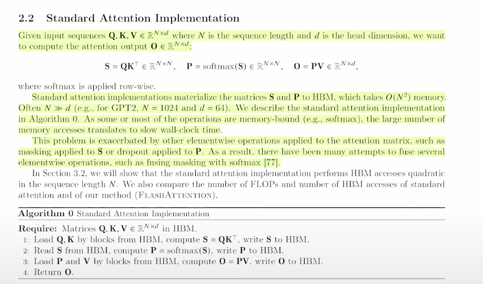
The Problem: Memory Bottleneck

Now, the issue with this is that HBM (High Bandwidth Memory), also called global memory, is very slow. HBM consists of the largest share—40 GB in H100, for example—but access is very slow (1.5 TB/s), so operations become memory-bound since they have to spend a lot of time waiting for I/O processes.

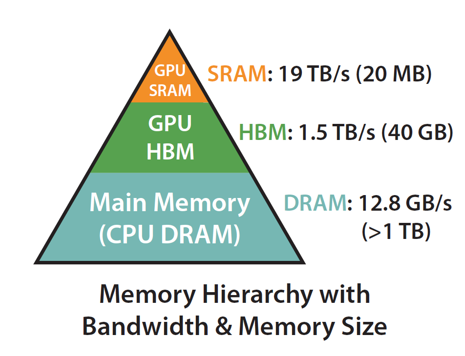
The Solution: Use Shared Memory

The solution is to calculate softmax and other memory-bound operations in shared memory, which is much smaller (20 MB) but faster (19 TB/s) and closer to the actual part that performs computation. So we will need to divide attention into smaller blocks that can reside in the shared memory.

2. Safe Softmax

Given a vector x, the softmax is defined as:

softmax(xi) = exi / Σj=1 to n exj

The Problem: Numerical Instability

But there's a problem: if the values of vector x are large, the exponent will explode, which makes it numerically unstable and cannot be represented with float32/16.

The Solution: Normalization Constant

We have a solution for it—add a constant to both numerator and denominator whose value is not equal to zero.

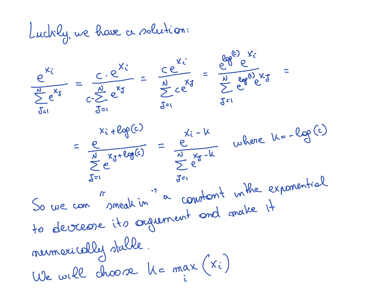
We take k = max(x_i), so now when k = max(x_i), then the numerator is e⁰ = 1, and for other numbers, e^{(some negative number)}, which is somewhere between 0 and 1, which can be easily represented by float32.

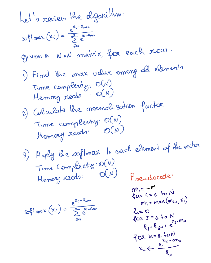
Algorithm Complexity

So now our algorithm becomes as shown in the image below:

1. Find max value among all elements → Time: O(N), Space: O(N)
2. Calculate the normalization factor → Time: O(N), Space: O(N)
3. Apply the softmax to each element of the vector → Time: O(N), Space: O(N)

Example

For x = [3, 2, 5]:

1. x_max = 5
2. L = e^(3-5) + e^(2-5) + e^(5-5)
3. x₁ = e^(3-5) / L, x₂ = e^(2-5) / L, x₃ = e^(5-5) / L

This basically means to apply a softmax to an N×N matrix, we need to load each of its elements 3 times, and it must be done sequentially. Do we have a better way?

3. Online Softmax

Pseudocode (Initial Approach)

m0 = -∞
for i = 1 to N:
    mi = max(mi-1, xi)

l0 = 0
for j = 1 to N:
    lj = lj-1 + e(xj - mn)

for k = 1 to N:
    xk = e(xk - mn) / ln

The Key Insight

Our approach now focuses on fusing step 1 and step 2 in one loop—that is, finding the max as well as calculating the normalization factor in one go. But the issue is we won't have global maxima yet, so we will have to use local maxima.

Example with Correction Factor

For x = [3, 2, 5, 1]:

• Step 1: max = 3, l₁ = e^(3-3)
• Step 2: max(2, 3) = 3, l₂ = l₁ + e^(2-3)
• Step 3: max(3, 5) = 5, l₃ = l₂ + e^(5-5)

But now l₃ computed is wrong since:

l3 = e(3-3) + e(2-3) + e(5-5)

Here it is using maxima as 3 for the first two values, so we will have to fix it using a correction factor on the fly:

l3 = l2 · e(3-5) + e(5-5)
    = (e(3-3) + e(2-3)) · e(3-5) + e(5-5)

where e^(3-5) is the correction factor

    = e(3-3+3-5) + e(2-3+3-5) + e(5-5)
    = e(3-5) + e(2-5) + e(5-5)

which is correct!

Final Pseudocode

m0 = -∞
l0 = 0

for i = 0 to n:
    mi = max(mi-1, xi)
    li = li-1 · e(mi-1 - mi) + e(xi - mi)

for k = 1 to n:
    xk = e(xk - mn) / ln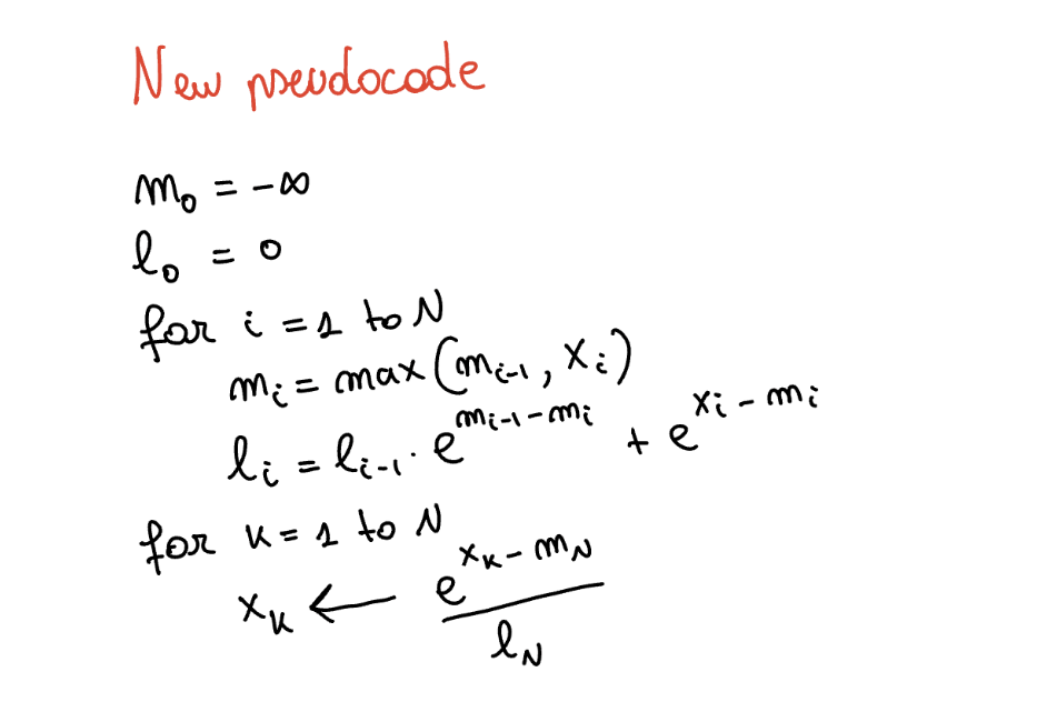

Proof

Proof that the final output is the same as the original can be found in the online softmax notes.

4. Block Matrix Multiplication

The Challenge of Parallelization

Consider matrix multiplication: C (M×N) = A (M×K) × B (K×N)

One way to parallelize could be using all cores equal to the number of elements, but as the number of elements grows, we can't parallelize. For example, if M×N is 100×100, we don't have ten thousand cores to parallelize. So we need a solution to parallelize this operation by using fewer cores than the number of elements in the matrix.

What is Block Matrix Multiplication?

Block matrix multiplication means you can divide the original matrix into smaller blocks and then conduct matrix multiplication operations on these small blocks.

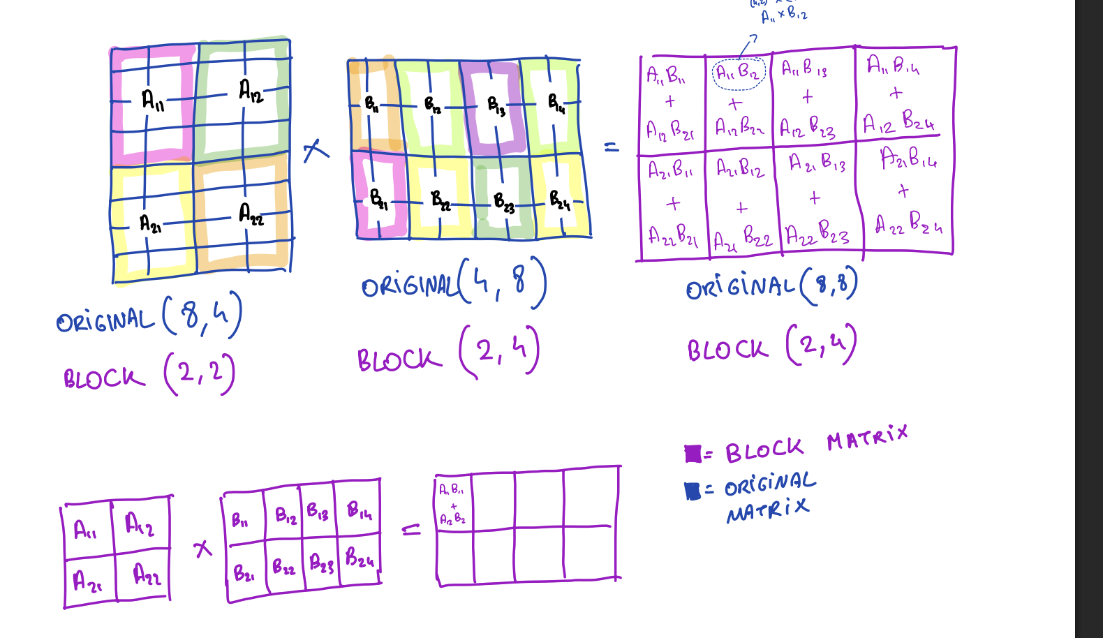
Example: 4×4 Matrices

Let's say you have two 4×4 matrices A and B. We divide each into 2×2 blocks:

A = [ A₁₁  A₁₂ ]     B = [ B₁₁  B₁₂ ]
    [ A₂₁  A₂₂ ]         [ B₂₁  B₂₂ ]

Each A_ij and B_ij is now a 2×2 submatrix.

The block product C = A × B is:

C = [ C₁₁  C₁₂ ]
    [ C₂₁  C₂₂ ]

where each block is computed like:

C₁₁ = A₁₁B₁₁ + A₁₂B₂₁
C₁₂ = A₁₁B₁₂ + A₁₂B₂₂
C₂₁ = A₂₁B₁₁ + A₂₂B₂₁
C₂₂ = A₂₁B₁₂ + A₂₂B₂₂

Just like scalar multiplication, but each "number" is a matrix block.

Why Should We Care?

Let's consider we want to do the operation:

S = Q·KT
P = softmax(S)
Output = P·V

For the time being, let's assume we don't want to do the softmax to simplify it, so our operation to be conducted is:

O = (Q·KT)·V

where dimensions of Q, K, V are N×d.

Block Dimensions

Dimensions of blocks can be anything as long as dimensions of the matrix made only of blocks should match in the matrix multiplication.

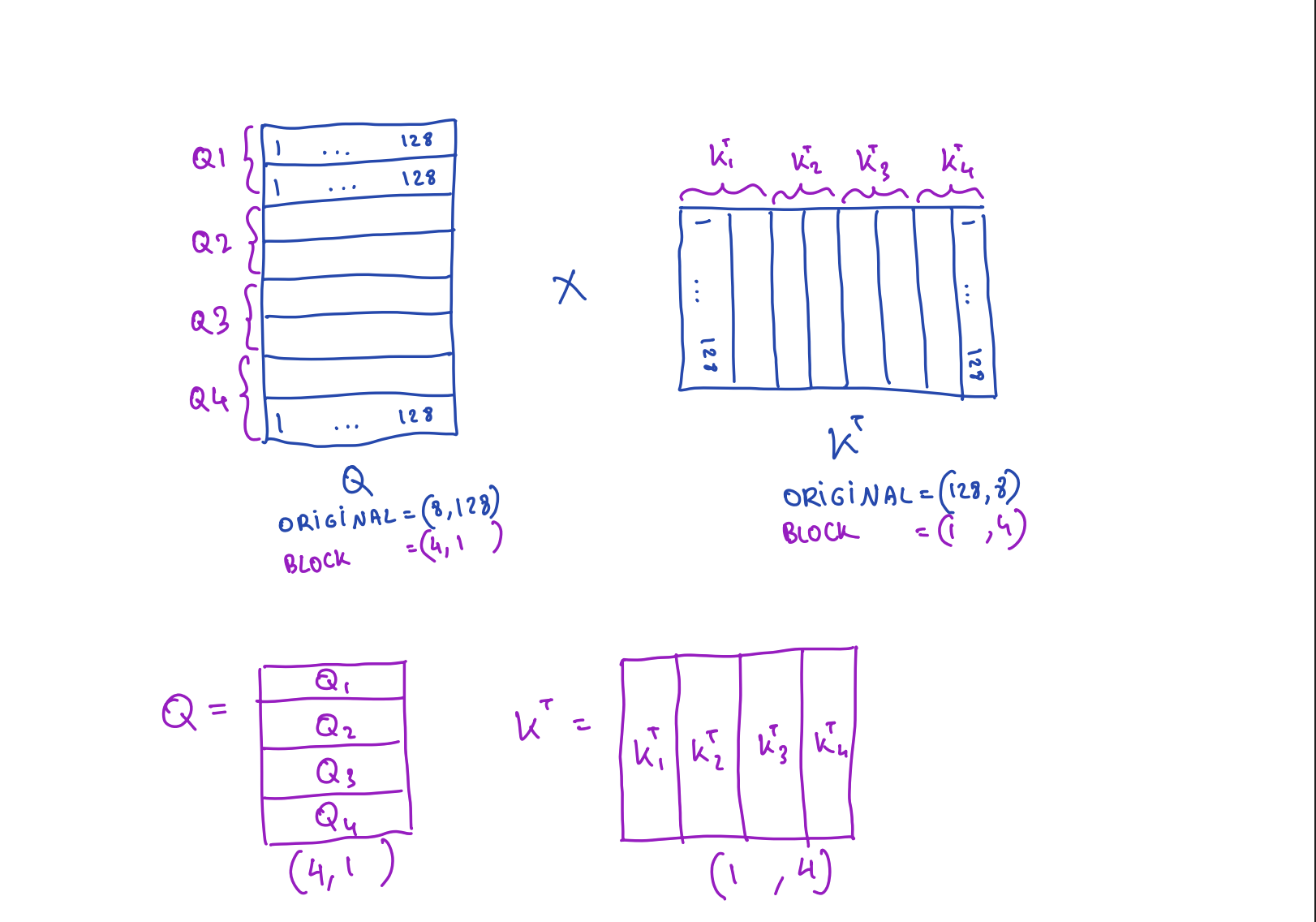
So let's say the dimensions are originally (8, 128) and we take the block size as (2, 128).

Step-by-Step Visualization

Original Matrix Shapes:

Q: (8, 128)
K: (8, 128)
V: (8, 128)

Block Structure (with block size 2×128):

Q: (8, 128)  →  Block structure: (4, 1)
                →  4 blocks of size (2, 128) arranged in 4 rows, 1 column

KT: (128, 8)  →  Block structure: (1, 4)
                →  4 blocks of size (128, 2) arranged in 1 row, 4 columns

V: (8, 128)  →  Block structure: (4, 1)
                →  4 blocks of size (2, 128) arranged in 4 rows, 1 column

Block-wise Computation:

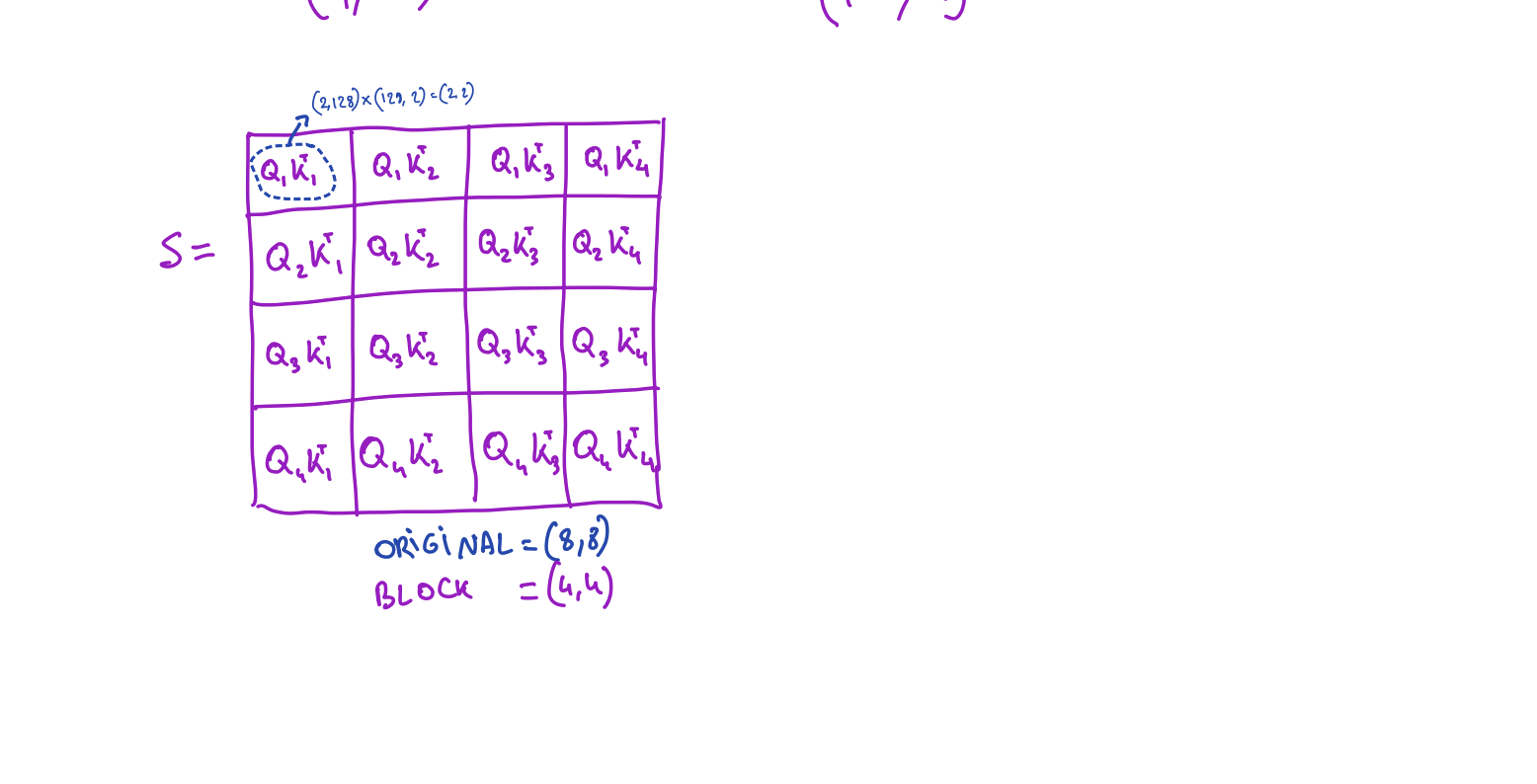
Step 1: S = Q · KT
        Block structure: (4, 1) × (1, 4) = (4, 4)
        Result: S has 4×4 = 16 blocks, each of size (2, 2)

Step 2: O = S · V
        Block structure: (4, 4) × (4, 1) = (4, 1)
        Result: O has 4×1 = 4 blocks, each of size (2, 128)

Individual Block Operations:

For each Qi block (2, 128):
    For each Kj block (2, 128):
        Sij = Qi · KjT
              = (2, 128) × (128, 2) = (2, 2)

    For each Vj block (2, 128):
        Oi contribution = Sij · Vj
                                   = (2, 2) × (2, 128) = (2, 128)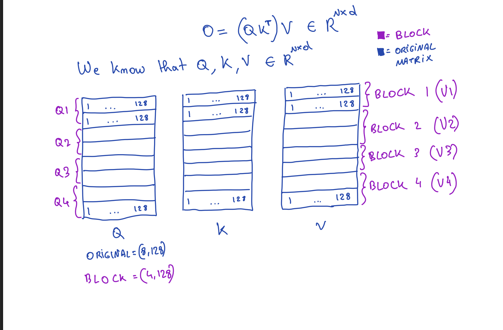

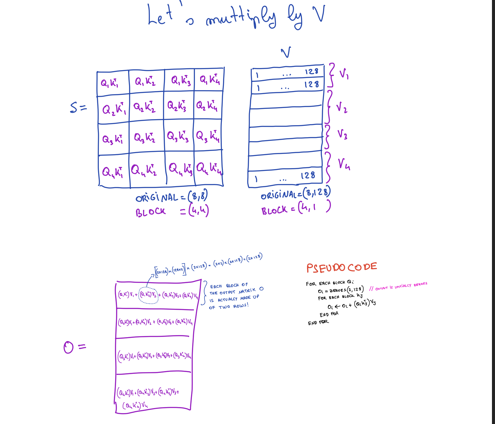
Pseudocode

for each block Qi:
    Oi = zeros(2, 128)
    for each block Kj:
        Oi = Oi + (Qi · KjT) · Vj
    end for
end for

5. Applying Softmax to Block Matrices

The Challenge

Now let's talk about softmax. We will apply softmax S* (where S* is softmax without the normalization denominator) to each element of the S matrix. But each element of the S matrix is not a single element. it's a matrix block itself!

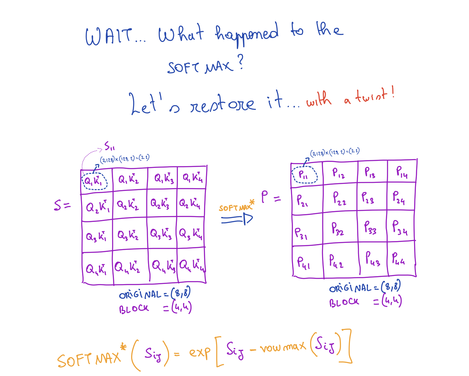
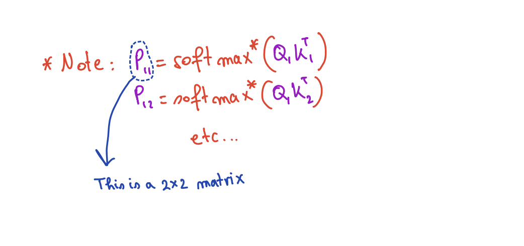
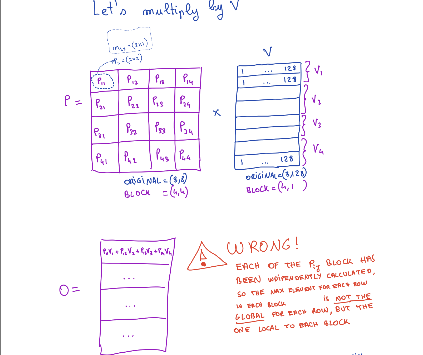
The Problem: Local vs Global Maxima

But there is a big problem with softmax it is not applied to the whole row. We were calculating S* at each block independently of other blocks in the same row, so it means that the maximum value we are using is actually the maximum value of the block and not the global maxima of the whole row.

So we need a way that if a maximum found in later steps is more than the one used in earlier steps, we need to correct it so that at last all blocks use the value of global maxima for that particular row. We have already talked about a solution earlier for this called online softmax.

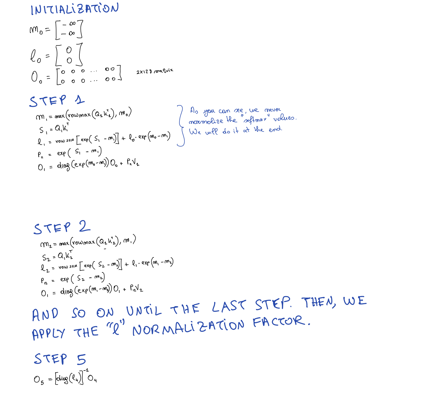
Processing Multiple Queries

Since our block size was (2, 128), which basically means we are processing 2 queries at a time, so we will have to find out two outputs:

Step 1 for first query:

• Find max m₁
• Apply S₁ = Q₁ · K₁^T
• l₁ = l₀ · e^{(m₀ - m₁)} + e^{(S₁ - m₀)}

Similarly for query 2

Then output:

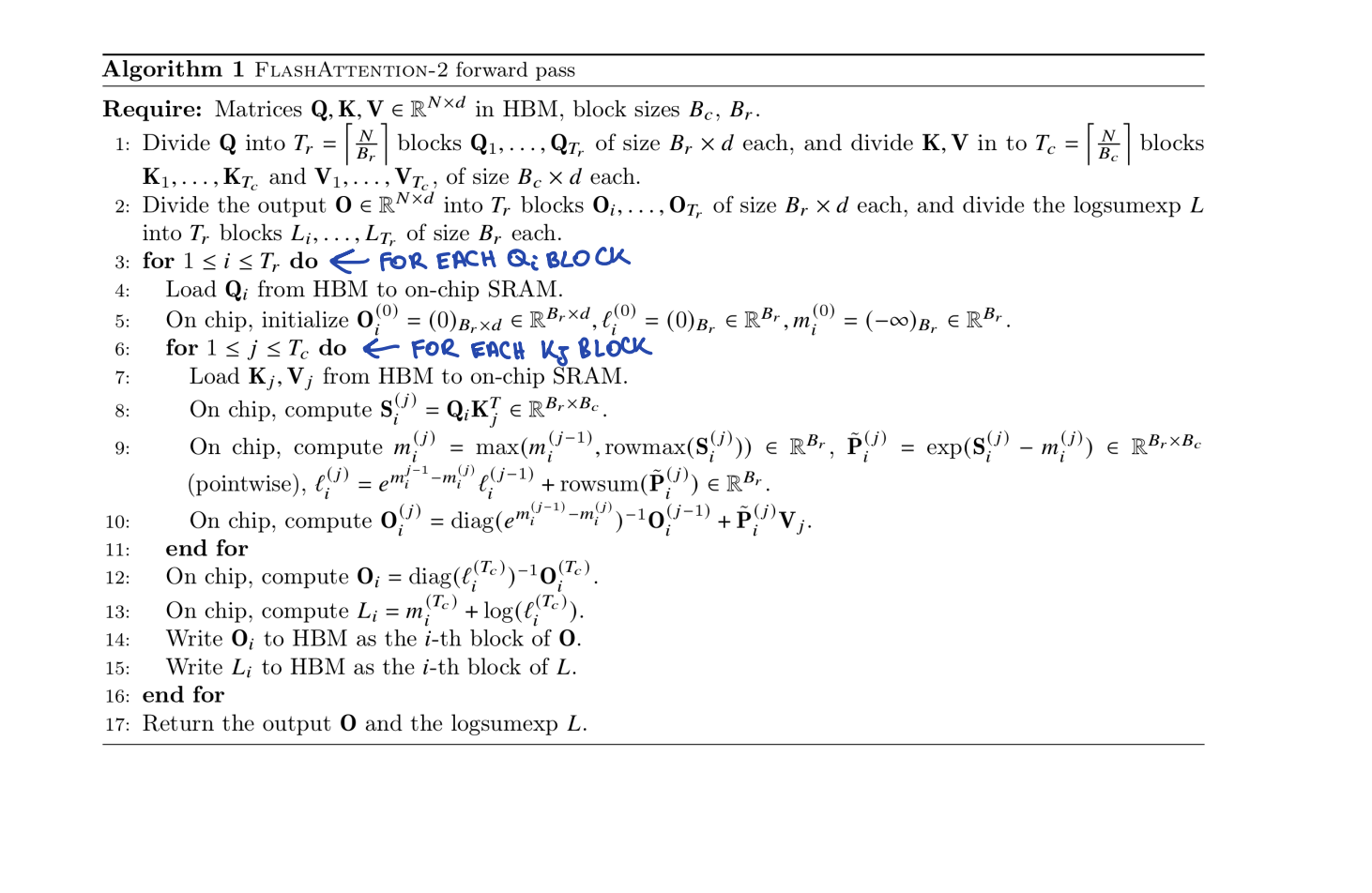
Oj = diag(e(prev_max - current_max))-1 · Oj-1 + Pj · Vj

Forward Pass: Flash Attention 2